1.5 Monopoly I: Behavior
Contents
Thursday, January 30, 2020 and Thursday, February 6, 2020
Overview
We begin looking at monopoly by discussing how a monopolist (as compared to a price-taking firm) chooses both its output and its price to maximize profits.
Slides
Appendix
Price Elasticity of Demand Refresher
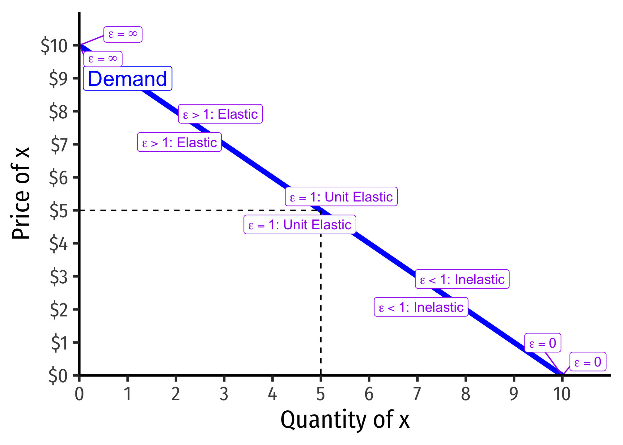
Price elasticity of demand measures how much (in %) quantity demanded changes in response to a (1%) change in price.
ϵq,p=%Δq%Δp=(Δqq)(Δpp)=ΔqΔp×pq=1slope×pq
| “Elastic” | “Unit Elastic” | “Inelastic” | |
|---|---|---|---|
| Intuitively: | Large response | Proportionate response | Little response |
| Mathematically: | |ϵqD,p|>1 | |ϵqD,p|=1 | |ϵqD,p|<1 |
| Numerator > Denominator | Numerator = Denominator | Numerator < Denominator | |
| A 1% change in p | More than 1% change in qD | 1% change in qD | Less than 1% change in qD |
Price elasticity of demand changes along the demand curve:

Determinants of Price Elasticity
What determines how responsive your buying behavior is to a price change?
- More (fewer) substitutes ⟹ more (less) elastic
- Larger categories of products (less elastic) vs. specific brand (more elastic)
- Necessities (less elastic) vs. luxuries (more elastic)
- Large (more elastic) vs. small (less elastic) portion of budget
- More (less) time to adjust ⟹ more (less) elastic
Derivation of the Lerner Index
Marginal revenue is strongly related to the price elasticity of demand, which is ED=ΔqΔp×pqI sometimes simplify it as ED=1slope×pq, where “slope” is the slope of the inverse demand curve (graph), since the slope is ΔpΔq=riserun.
We derived marginal revenue (in the slides) as:
MR(q)=p+ΔpΔqq
Firms will always maximize profits where:
MR(q)=MC(q)Profit-max outputp+(ΔpΔq)q=MC(q)Definition of MR(q)p+(ΔpΔq)q×pp=MR(q)pMultiplying the left by pp (i.e. 1)p+(ΔpΔq×qp)⏟1ϵ×p=MC(q)Rearranging the leftp+1ϵ×p=MC(q)Recognize price elasticity ϵ=ΔqΔp×pqp=MC(q)−1ϵpSubtract 1ϵp from both sidesp−MC(q)=−1ϵpSubtract MC(q) from both sidesp−MC(q)p=−1ϵDivide both sides by p
The left side gives us the fraction of price that is markup (p−MC(q)p), and the right side shows this is inversely related to price elasticity of demand.