Firm Decisions in the Long Run I
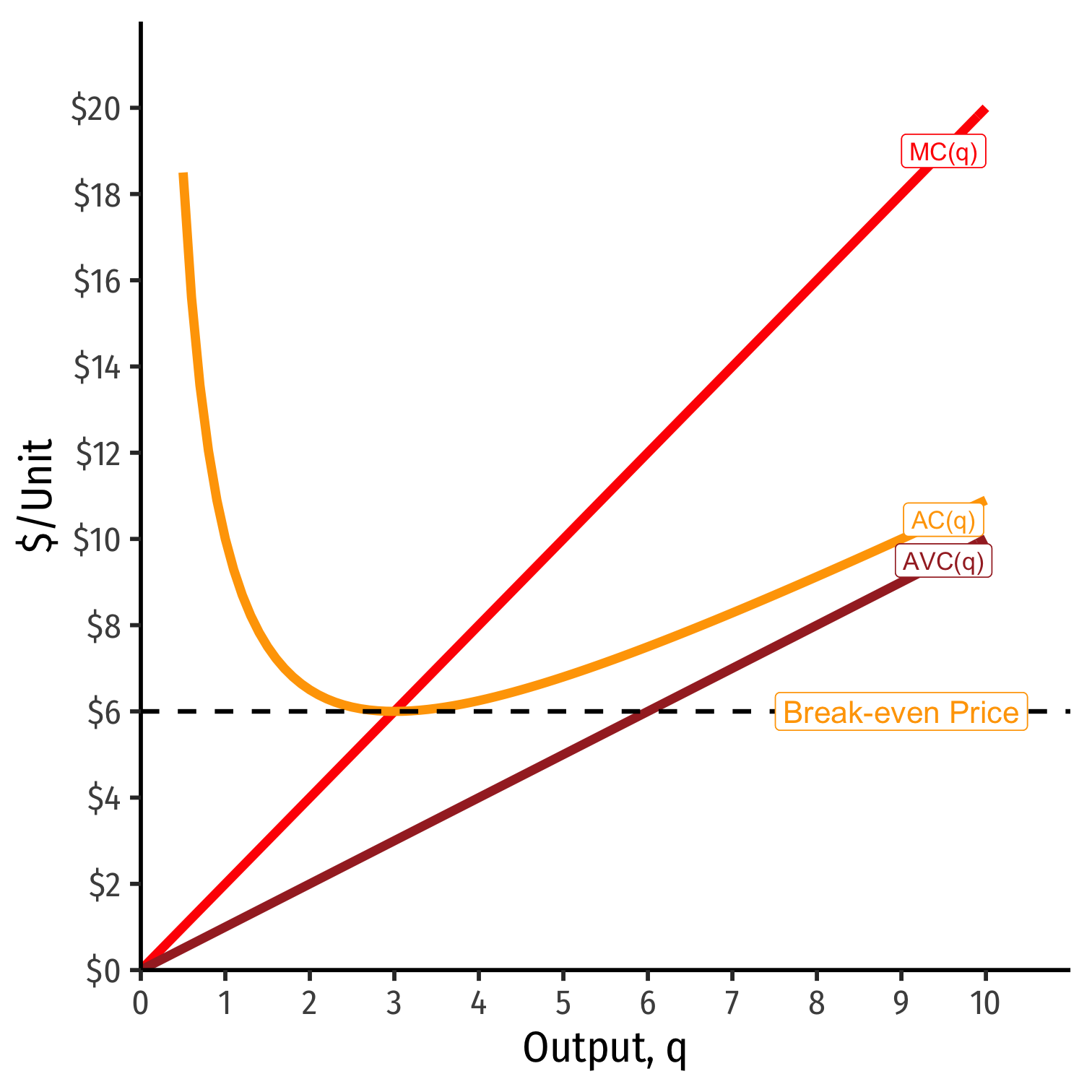
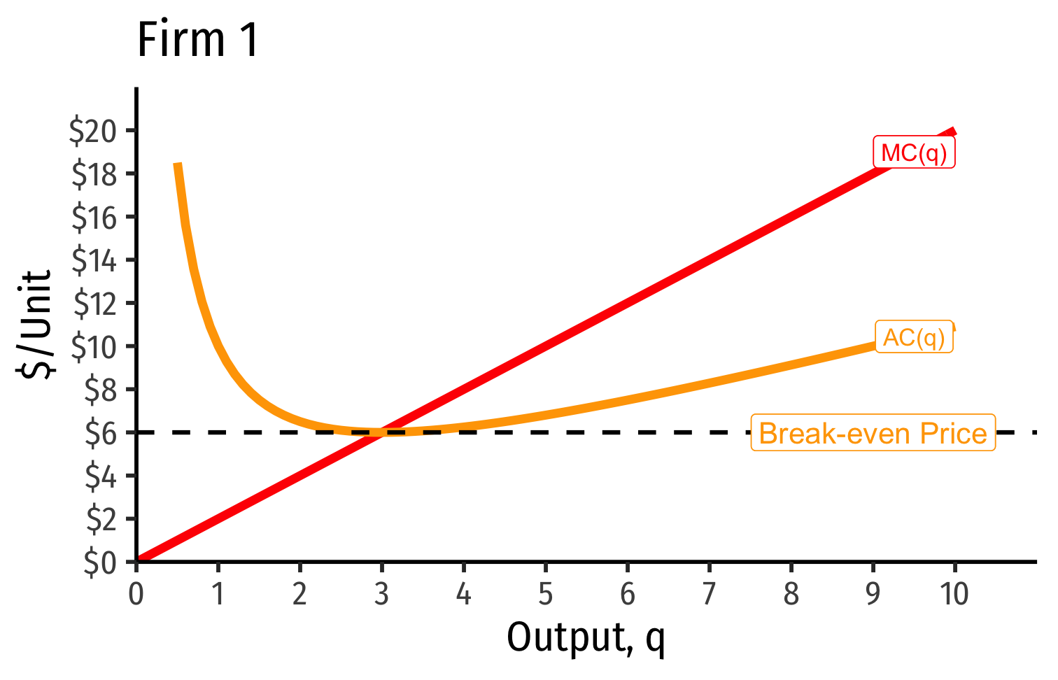
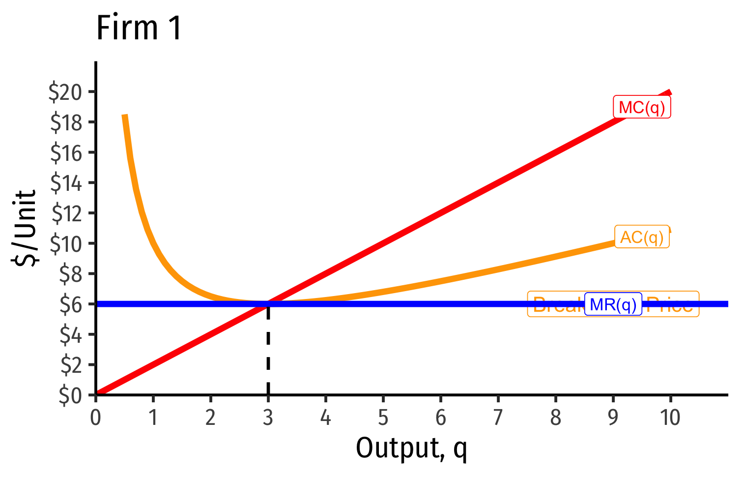
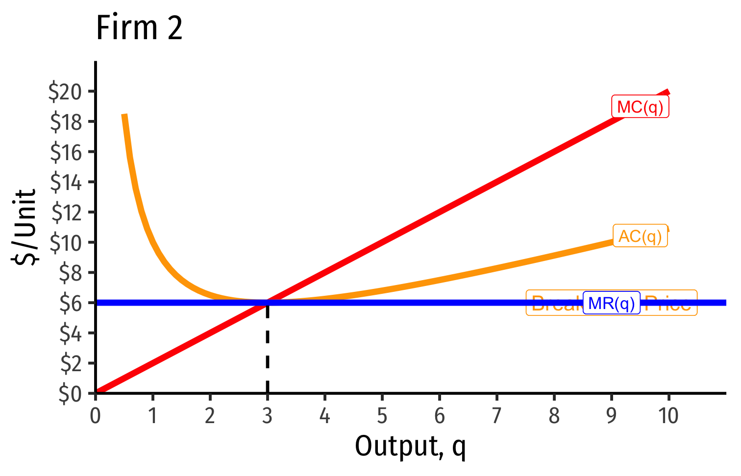
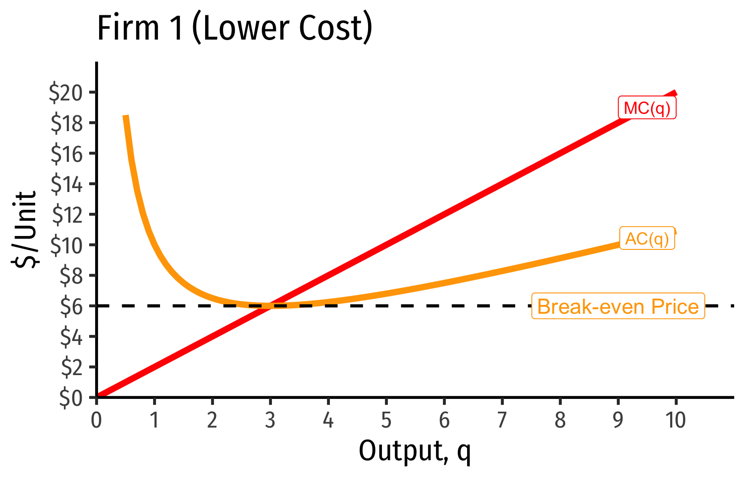
AC(q)min at a market price of $6
At $6, the firm earns "normal economic profits"
At any market price below $6.00, firm earns losses
- Short Run: firm shuts down if p<AVC(q)
At any market price above $6.00, firm earns "supernormal profits"
Firm Supply Decisions in the Short Run vs. Long Run
Short run: firms that shut down (q∗=0) stuck in market, incur fixed costs π=−f
Long run: firms earning losses (π<0) can exit the market and earn π=0
- No more fixed costs, firms can sell/abandon f at q∗=0

Firm Supply Decisions in the Short Run vs. Long Run
Short run: firms that shut down (q∗=0) stuck in market, incur fixed costs π=−f
Long run: firms earning losses (π<0) can exit the market and earn π=0
- No more fixed costs, firms can sell/abandon f at q∗=0
Entrepreneurs not currently in market can enter and produce, if entry would earn them π>0

Firm's Long Run Supply: Visualizing
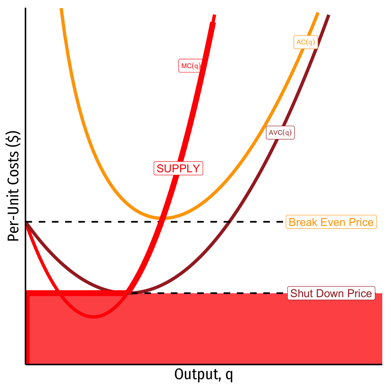
When p<AVC
Profits are negative
Short run: shut down production
- Firm loses more π by producing than by not producing
Long run: firms in industry exit the industry
- No new firms will enter this industry
Firm's Long Run Supply: Visualizing
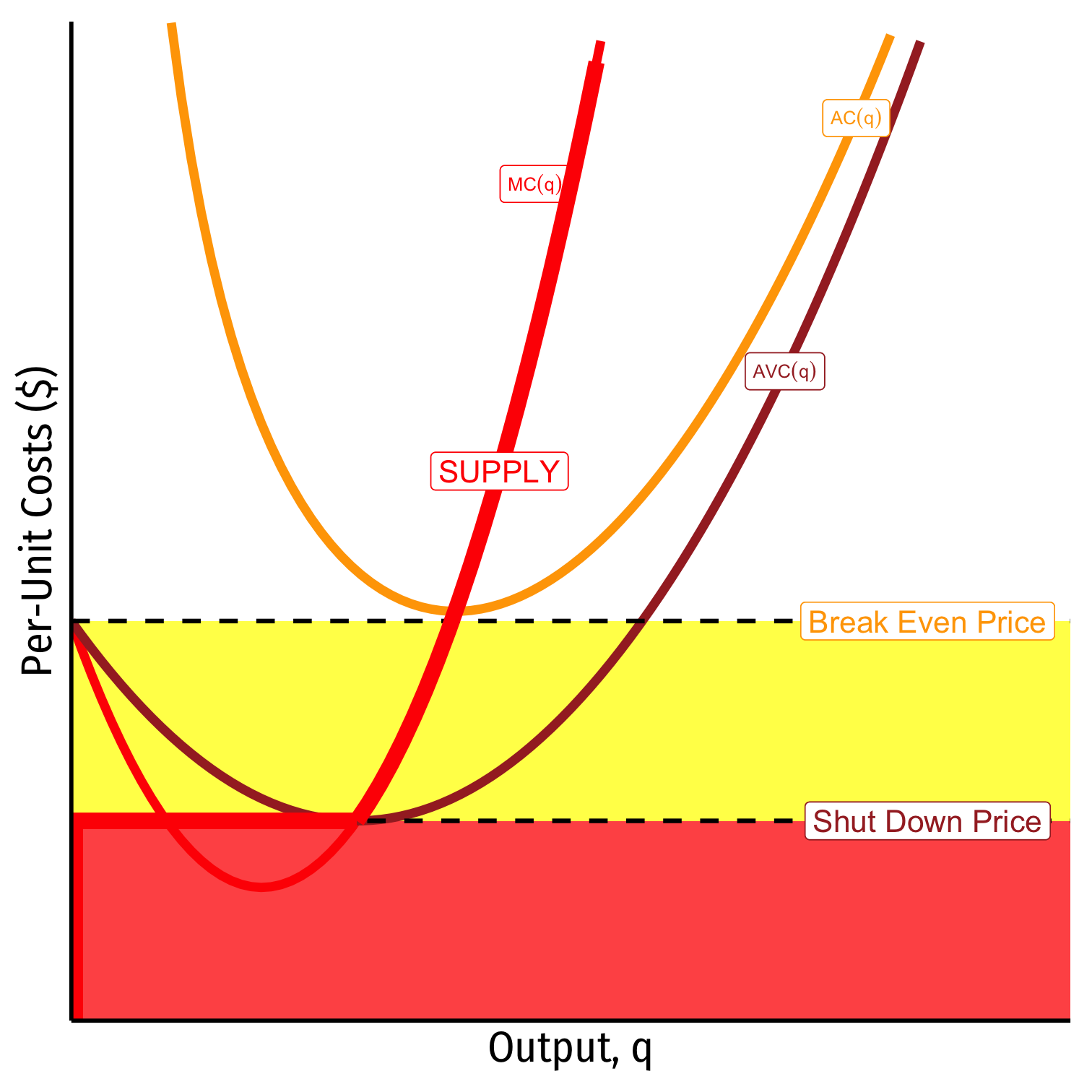
When AVC<p<AC
Profits are negative
Short run: continue production
- Firm loses less π by producing than by not producing
Long run: firms in industry exit the industry
- No new firms will enter this industry
Firm's Long Run Supply: Visualizing
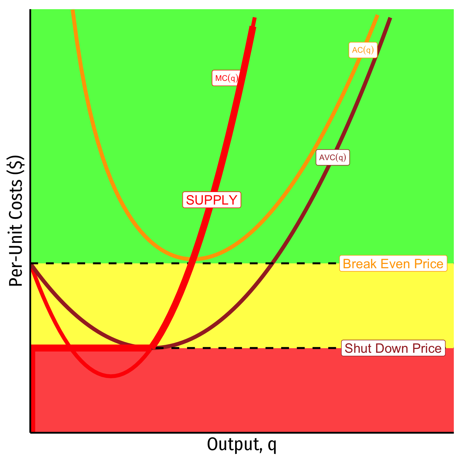
When AC<p
Profits are positive
Short run: continue production
- Firm earn profits
Long run: firms in industry stay in industry
- New new firms will enter this industry
Exit, Entry, and Long Run Industry Equilibrium I
Now we must combine optimizing individual firms with market-wide adjustment to equilibrium
Since π=[p−AC(q)]q, in the long run, profit-seeking firms will:
- Enter markets where p>AC(q)
Exit, Entry, and Long Run Industry Equilibrium I
Now we must combine optimizing individual firms with market-wide adjustment to equilibrium
Since π=[p−AC(q)]q, in the long run, profit-seeking firms will:
- Enter markets where p>AC(q)
- Exit markets where p<AC(q)
Exit, Entry, and Long Run Industry Equilibrium II
- Long-run equilibrium: entry and exit ceases when p=AC(q) for all firms, implying normal economic profits of π=0

Exit, Entry, and Long Run Industry Equilibrium II
Long-run equilibrium: entry and exit ceases when p=AC(q) for all firms, implying normal economic profits of π=0
Zero Profits Theorem: long run economic profits for all firms in a competitive industry are 0
Firms must earn an accounting profit to stay in business
Industry Supply Curves (Identical Firms)

Industry Supply Curves (Identical Firms)
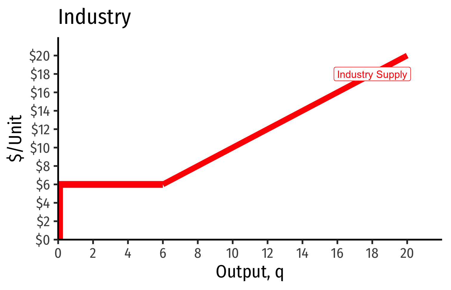
- Industry supply curve is the horizontal sum of all individual firm's supply curves
- Which are each firm's marginal cost curve above its breakeven price
Industry Supply Curves (Identical Firms)
- Industry demand curve (where equal to supply) sets market price, demand for firms
Industry Supply Curves (Identical Firms)


Short Run: each firm is earning profits p>AC(q)
Long run: induces entry by firm 3, firm 4, ⋯, firm n
Industry Supply Curves (Identical Firms)
Short Run: each firm is earning profits p>AC(q)
Long run: induces entry by firm 3, firm 4, ⋯, firm n
- Long run industry equilibrium:
Industry Supply Curves (Identical Firms)
Short Run: each firm is earning profits p>AC(q)
Long run: induces entry by firm 3, firm 4, ⋯, firm n
Long run industry equilibrium: p=AC(q)min, π=0 at p= $6; supply becomes more elastic
Back to Zero Profits
Recall, we've defined a firm as a completely replicable recipe (production function) of resources
Anyone can enter market, buy required factors, and produce q∗ at market price p and earn the market rate of π
Let's start considering some realistic differences between firms

Industry Supply Curves (Different Firms) I
- Firms may have different costs due to differences in:
- Managerial talent
- Worker talent
- Location
- First-mover advantage
- Technological secrets/IP
- License/permit access
- Political connections
- Lobbying

Industry Supply Curves (Different Firms) II
Industry Supply Curves (Different Firms) II
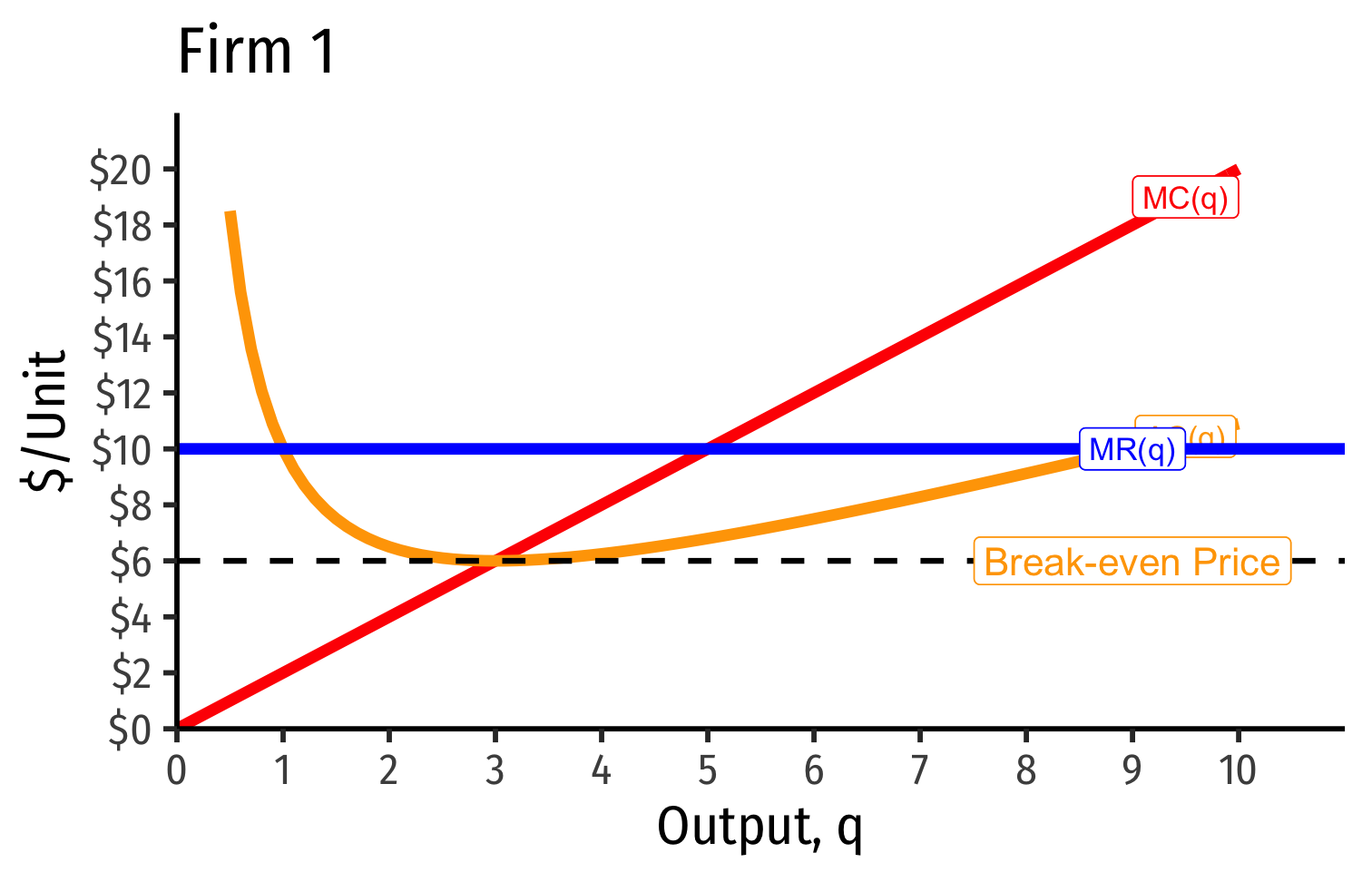
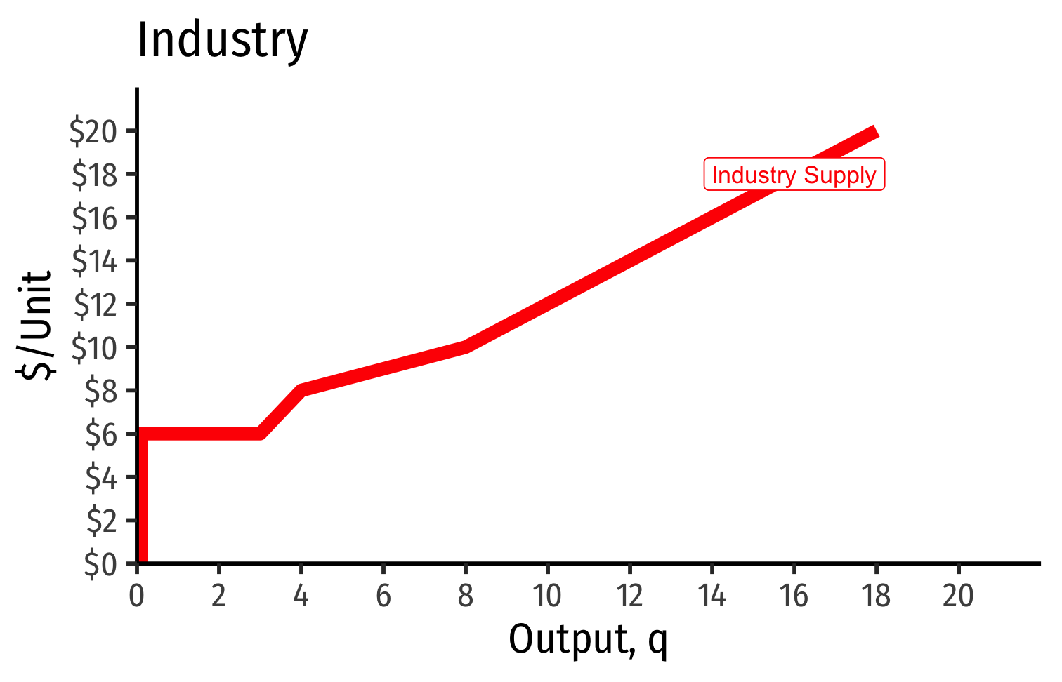
- Industry supply curve is the horizontal sum of all individual firm's supply curves
- Which are each firm's marginal cost curve above its breakeven price
Industry Supply Curves (Different Firms) II
Industry Supply Curves (Different Firms) II
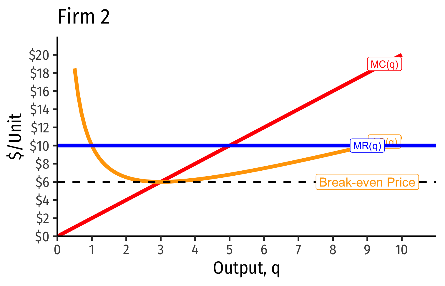
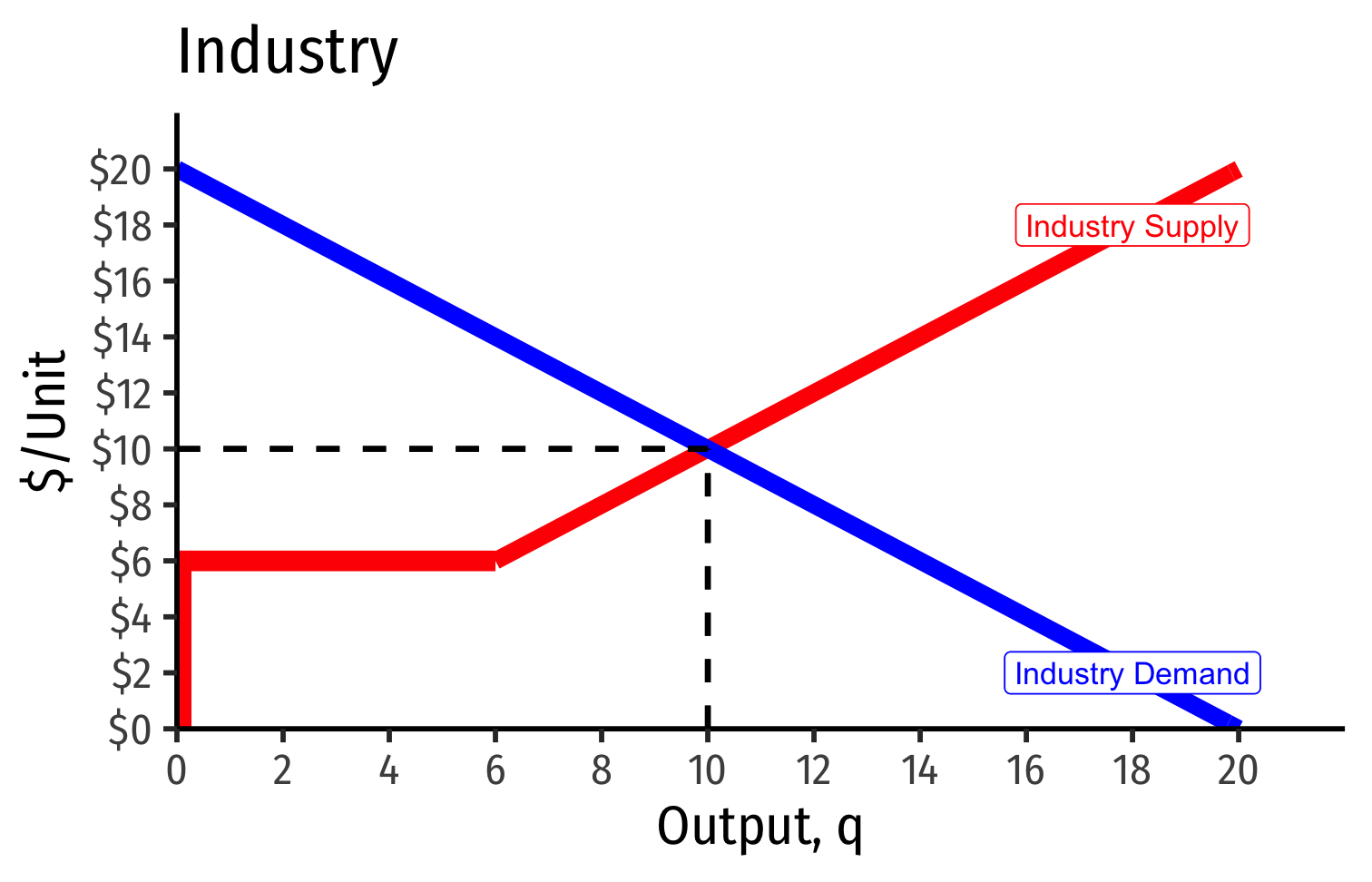
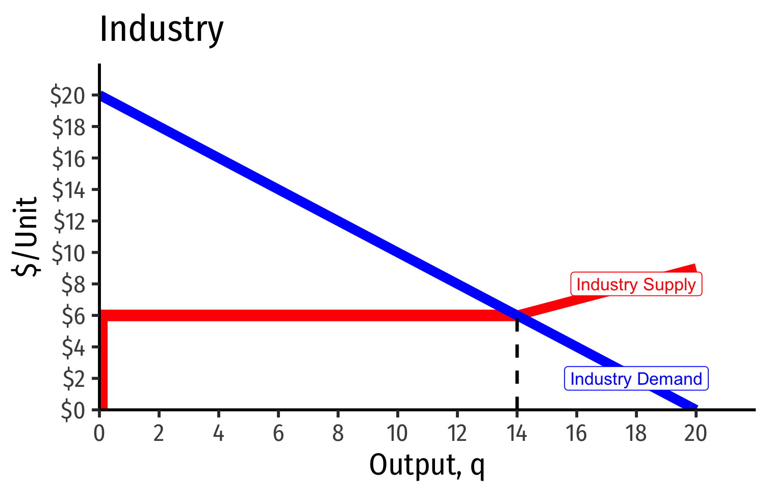
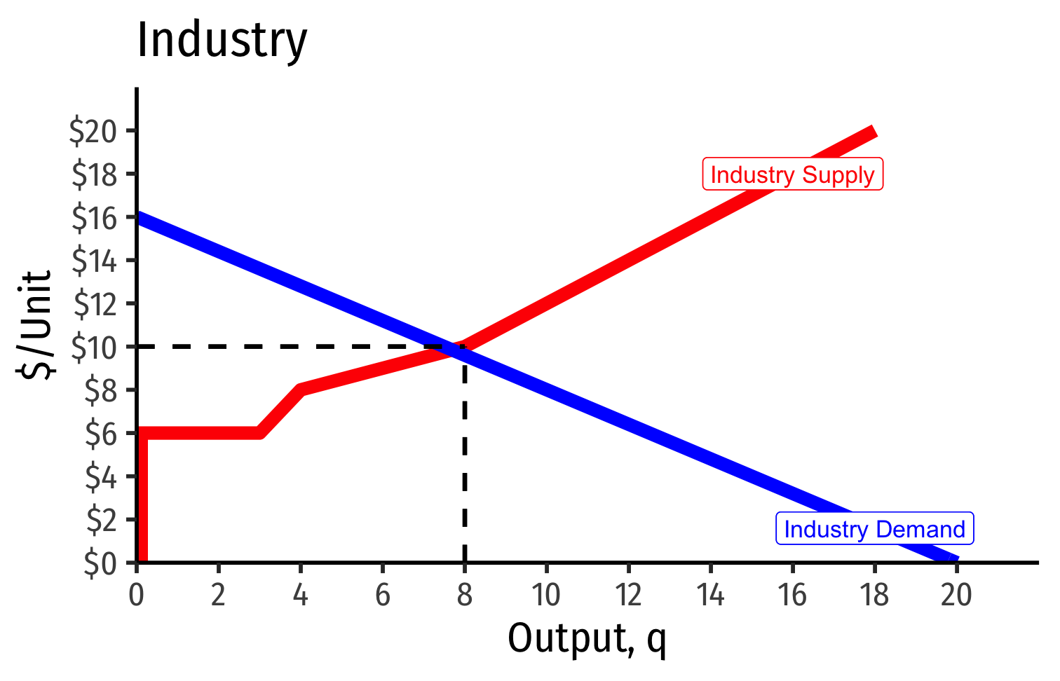
- Industry demand curve (where equal to supply) sets market price, demand for firms
Industry Supply Curves (Different Firms) II
- Industry demand curve (where equal to supply) sets market price, demand for firms
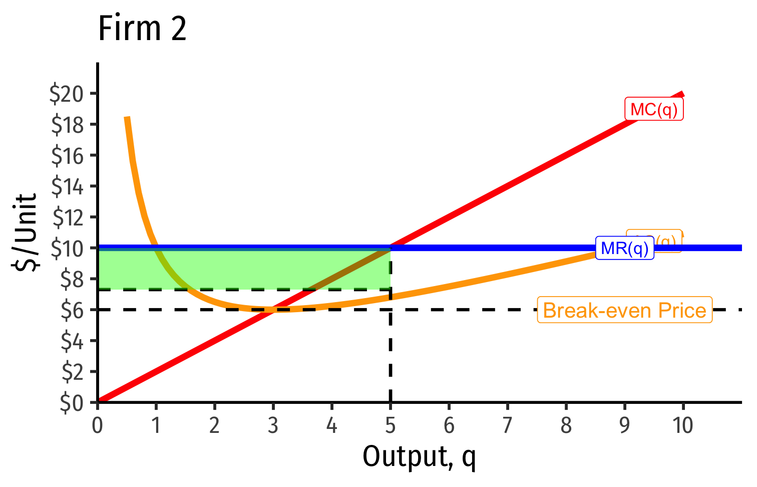
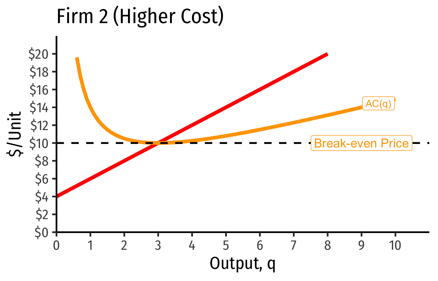
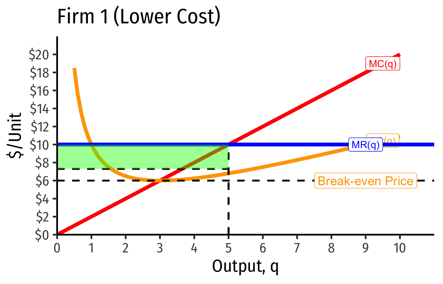
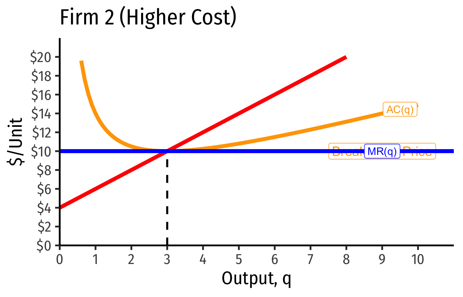
- Long run industry equilibrium: p=AC(q)min, π=0 for marginal (highest cost) firm (Firm 2)
Industry Supply Curves (Different Firms) II
- Industry demand curve (where equal to supply) sets market price, demand for firms
- Long run industry equilibrium: p=AC(q)min, π=0 for marginal (highest cost) firm (Firm 2)
- Firm 1 (lower cost) appears to be earning profits...
Economic Rents and Zero Economic Profits I

- With differences between firms, long-run equilibrium p=AC(q)min of the marginal (highest-cost) firm
- If p>AC(q) for that firm, would induce more entry into industry!
Economic Rents and Zero Economic Profits I
"Inframarginal" (lower-cost) firms earn economic rents
- returns higher than their opportunity cost (what is needed to bring them into this industry)
Economic rents arise from relative differences between firms
- actually using different inputs!
Economic Rents and Zero Economic Profits III
Some factors are relatively scarce in the economy
- (talent, location, secrets, IP, licenses, being first, political favoritism)
Inframarginal firms that use these scarce factors gain a cost-advantage
It would seem these firms earn profits as other firms have higher costs...
- ...But what will happen to the prices for the scarce factors?
Economic Rents and Zero Economic Profits IV

Rival firms willing to pay for rent-generating factor to gain advantage
Competition over acquiring the scarce factors push up their prices
Rents are included in the opportunity cost (price) for inputs
- Must pay a factor enough to keep it out of other uses
Economic Rents and Zero Economic Profits IV
Economic rents ≠ profits!
- Rents actually reduce profits!
Firm does not earn the rents, they raise firm's costs and squeeze out profits!
Scarce factor owners (workers, landowners, inventors, etc) earn the rents as higher income for their scarce services (wages, rents, interest, royalties, etc).
Recall: Accounting vs. Economic Point of View
Recall "economic" point of view:
Producing your product pulls scarce resources out of other productive uses in the economy
Profits attract resources to be pulled out of other uses
Losses repel resources to be pulled away to other uses
Zero profits ⟹ resources should stay where they are
- Optimal use of resources!


Market-Clearing Prices
- Supply and demand set the market-clearing price for all units exchanged (bought and sold)
Consumer Surplus I
Demand function measures how much you would hypothetically be willing to pay for various quantities
- "reservation price"
You often actually pay (the market-clearing price, p∗) a lot less than your reservation price
The difference is consumer surplus
CS=WTP−p∗
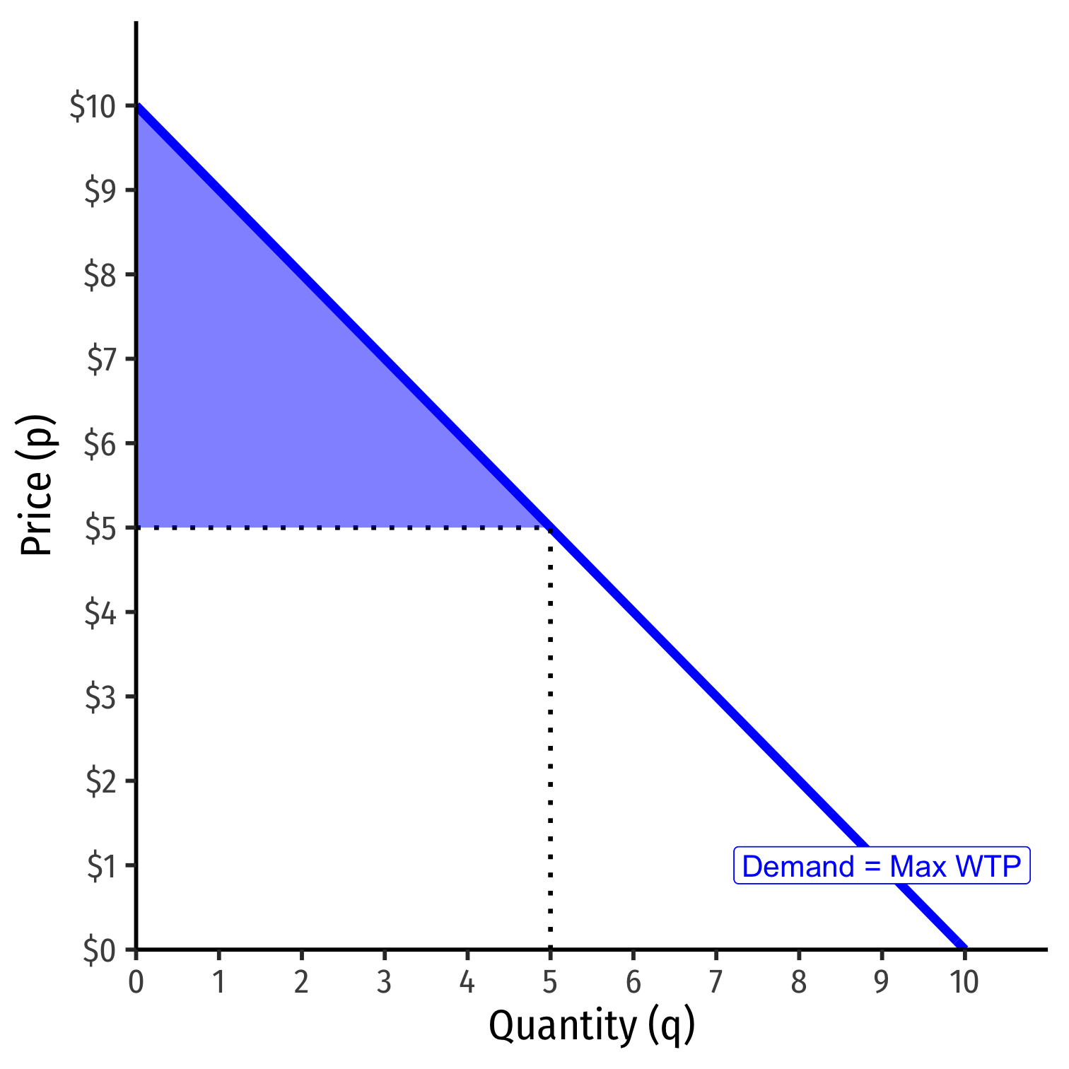
Consumer Surplus II
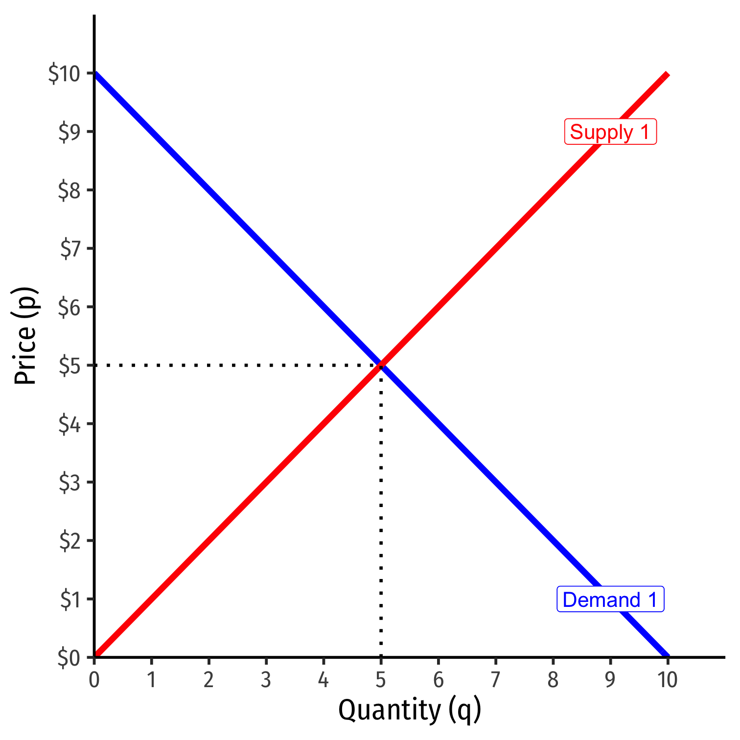
CS=12bhCS=12(5−0)($10−$5)CS=$12.50

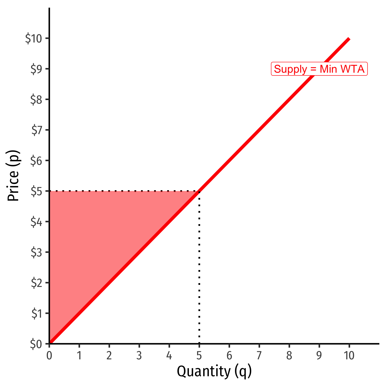
Producer Surplus I
Supply function measures how much you would hypothetically be willing to accept to sell various quantities
- "reservation price"
You often actually receive (the market-clearing price, p∗) a lot more than your reservation price
The difference is producer surplus
PS=p∗−WTA
Market Efficiency in Competitive Equilibrium I
Allocative efficiency: resources are allocated to highest-valued uses
- Goods produced up to the point where MB=MC (p=MC)
All potential gains from trade are fully exhausted
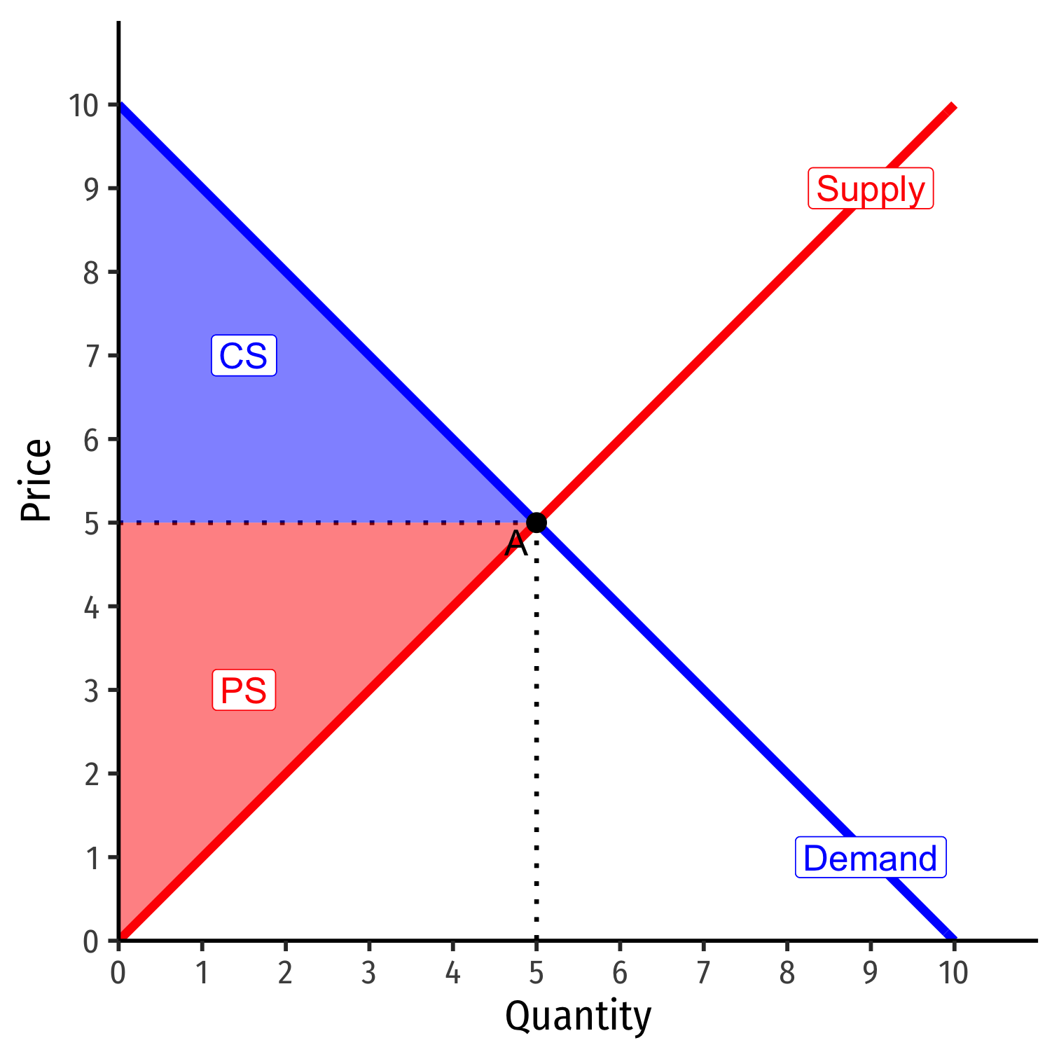
Market Efficiency in Competitive Equilibrium II
Economic surplus = Consumer surplus + Producer surplus
Maximized in competitive equilibrium
Resources flow away from those who value them the lowest to those that value them the highest
The social value of resources is maximized by allocating them to their highest valued uses!
